Vector Databases from First Principles: Why Your Postgres Slows to a Crawl When You Add "Meaning"

Source: System Design One (Issue #141) · Authors: Maxine Meurer & Neo Kim · Date: Apr 25, 2026 · Original article

Note: The original post is paywalled. This summary covers the freely accessible portion (the problem statement, why traditional DBs fail, the storage layer, and the HNSW indexing layer). The query layer, production realities, and decision framework are behind the paywall and not included.

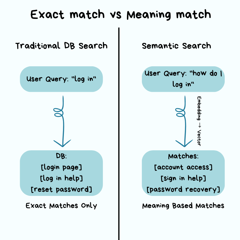
The setup: search that "understands meaning"

You build a search feature on a normal relational database. It works fine — until product asks for semantic search: a user typing "how do I log in" should also surface results about "account access" and "sign in", even though none of those words match. That's a fundamentally different problem from what your relational database was built for.

Everything that made your DB fast — B-tree indexes, WHERE clauses, keyword matching — is built around finding exact values. Semantic search doesn't have exact values; it has similar meanings. So your DB falls back to its only option: scan every row, compare it to your query, and rank. Milliseconds become seconds. The DB isn't broken — it's doing literally what you asked.

This is the gap vector databases exist to fill.

Why traditional databases struggle with embeddings

Relational DBs shine at exact matches and ranges. WHERE user_id = 12345 is fast because the index lets the engine jump to the right row, the same way you flip to the right section of a dictionary instead of reading every page. WHERE created_at > '2026-01-01' works the same way for ranges.

Embeddings break this model because there is no exact value to look up.

An embedding is a list of numbers that represents the meaning of a piece of text. An AI model converts words, sentences, or paragraphs into these numbers, and similar meanings produce numerically similar vectors.

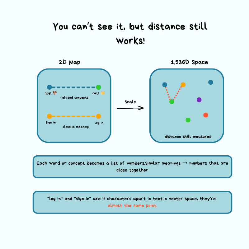
Think of it like a map: latitude + longitude give you a point in 2D space. An embedding from a model like OpenAI's text-embedding-3-small gives you a point in 1,536-dimensional space. Similar text lands close together; unrelated text lands far apart.

A concrete example

You have a document database. Each document is split into chunks (think: cutting a book into individual paragraphs so each can be searched independently). Each chunk is embedded into a 1,536-dim vector. The flow at query time:

1. User submits a search query.
2. App converts the query into a vector using the same embedding model.
3. You need to find the chunks "most similar" to that query vector.

Without a specialized index, the only way to find "most similar" is brute force: compute the distance from the query vector to every chunk vector, sort, return the top results.

The Times Square analogy

Imagine standing in Times Square needing the 10 closest coffee shops, with no map and no list. Your only option:

1. Walk to every building.
2. Check if it's a coffee shop.
3. Measure the distance.
4. Keep a running top-10.

10,000 buildings → check 10,000. 10 million → check 10 million.

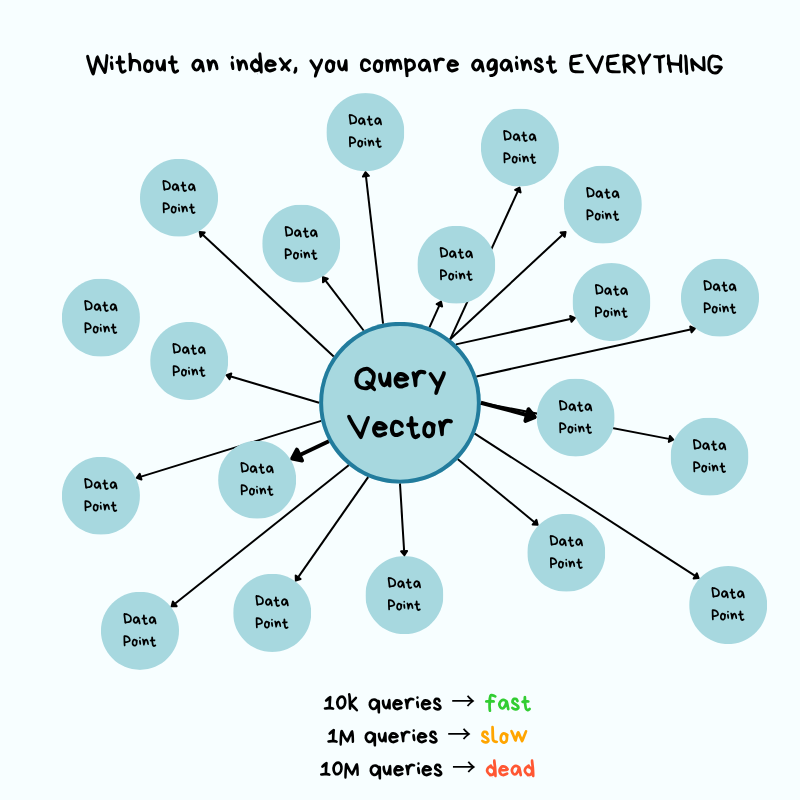
That's $O(n)$ — time grows linearly with dataset size. Concretely: if each distance calc takes 0.0001 s, then:

• 10,000 chunks → 1 second per query. Tolerable.
• 10 million chunks → 1,000 seconds (~16 minutes) per query.
• Throw 100 QPS at it from real users and the system grinds to a halt.

The "similar songs" intuition

Finding a song similar to one you like isn't a name lookup; you'd have to compare it to every other song across many characteristics — tempo, key, energy, mood. More songs → more work. Vector search is the same, except you're comparing across 1,536 dimensions simultaneously, on text. Without specialized techniques, the math just doesn't scale.

Where pgvector fits

pgvector is a Postgres extension that adds vector search to a database you probably already run. For fewer than ~100,000 vectors with moderate query volume, it works well and saves you from operating a second database. As you push into the millions of vectors with tighter latency budgets, you hit the limits of a general-purpose engine on this specific workload.

The takeaway isn't "embeddings = dedicated vector DB." It's: know when the operational trade-offs tip in favor of dedicated infrastructure.

The real question vector databases answer:

How do you find approximate nearest neighbors in high-dimensional space without comparing against every vector, and still return results that are "good enough"?

The answer is a class of index structures that trade a small amount of accuracy for massive speed gains.

Architecture: how a vector database works under the hood

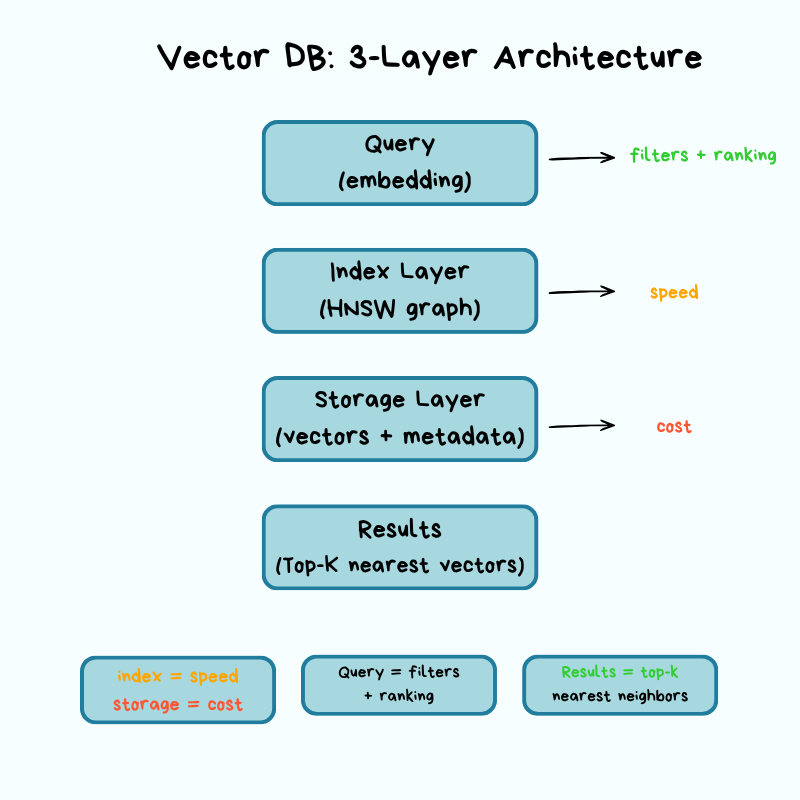
A vector DB has three layers — storage, index, query — and each layer forces explicit trade-offs across cost, latency, accuracy, and scalability.

Storage layer: where vectors live

Vectors are big. A single 1,536-dim vector at 32-bit floats is 6 KB. Multiply by millions and storage and (more importantly) memory costs balloon. The storage layer's job is to keep them on disk and in RAM efficiently while preserving accuracy.

Quantization is the most common trick. It reduces the precision of each dimension:

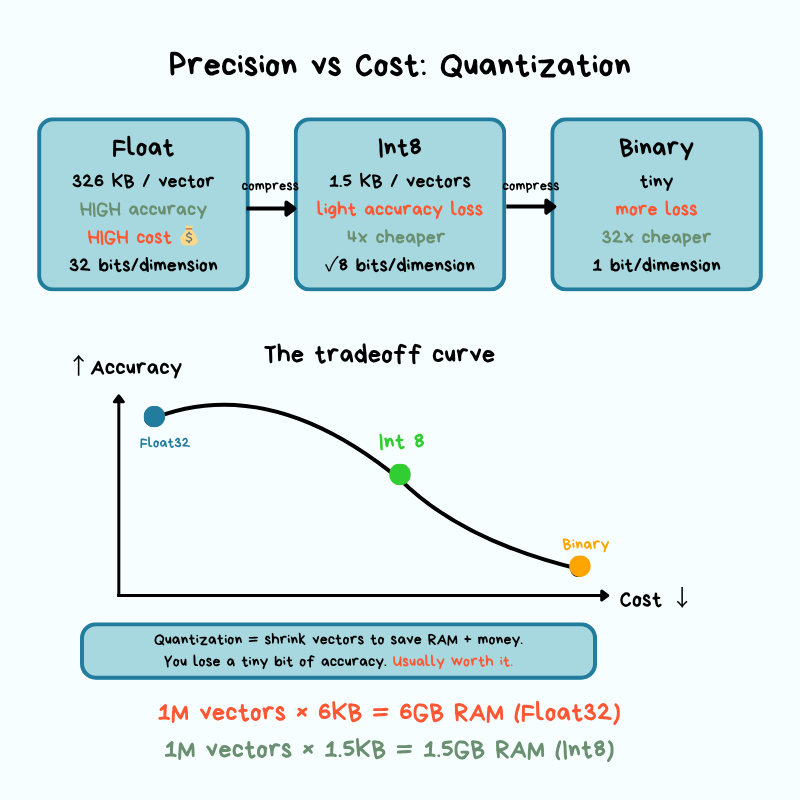
• Scalar quantization: store each dimension as an 8-bit integer instead of a 32-bit float (~4× shrink).
• Binary quantization: even more aggressive — represent dimensions as bits.

The cost is approximation error — the gap between the compressed representation and the original. When you round numbers to save space, your distance calculations get slightly less precise. In practice, that means you might occasionally miss the truly closest match, but most applications never notice.

Memory vs. disk is the other big lever:

• Maximum query speed → keep the index in RAM. Expensive at scale.
• Tiered storage — hot vectors in RAM, cold ones on disk.
• Hybrid — index structure in RAM, raw vectors fetched from disk when needed.

These choices directly shape your cost and your tail latency (p99).

Operationally, before you pick a vector DB, get answers to:

• What happens if a node crashes mid-write?
• How long does index rebuild take after a restart?
• Are vectors written to disk synchronously or asynchronously?

These are the difference between "minor blip" and "major incident."

Indexing layer: HNSW (the graph that replaces O(n))

The dominant production algorithm is HNSW — Hierarchical Navigable Small World. Worth understanding conceptually even if you'll never implement it.

The core idea borrows from "small world" networks — the same intuition behind "six degrees of separation": from any person on the planet, you're only a few hops away from any other. HNSW builds a multi-layer graph where similar vectors are connected as neighbors. To answer a query, it starts at the top (sparse) layer, walks toward your query by following edges to similar neighbors, and drops down through layers until it lands on the closest matches at the bottom.

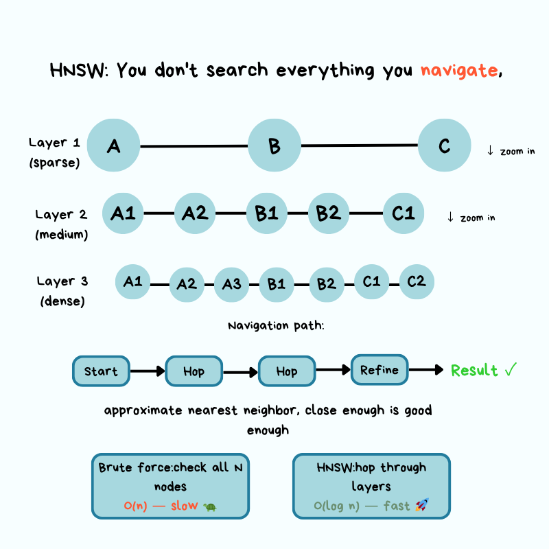
The Google Maps analogy

Imagine navigating from New York to a specific coffee shop in San Francisco:

• Top layer (zoomed out): From New York, you only see major waypoints. You pick the West Coast direction and follow long-range connections to California. You're not considering every city in America.
• Middle layers (zooming in): Now in California, you narrow to the SF Bay Area, hopping between nearby regions. Still not checking every street, just neighborhoods that point toward the target.
• Bottom layer (street level): You're in the right neighborhood and follow the last few connections to the exact address — the most similar document chunks.

At every zoom level you only follow connections that take you closer. That's how HNSW collapses an $O(n)$ scan into something dramatically faster — it builds a navigation structure that lets you skip large portions of the map heading the wrong way.

The two knobs: M and ef

HNSW exposes a speed-vs-accuracy trade-off via two parameters:

• M (max connections): how many neighbors each vector links to in the graph.
• ef (exploration factor): how many neighbors to examine during a search.

Higher values → better recall, but slower queries and a bigger index. Lower values → faster queries, but you might miss relevant results. In production you tune these against your latency budget and accuracy tolerance.

Index build is expensive

Inserting a vector requires distance calculations and updating graph edges, so bulk index builds typically run offline or during low-traffic windows. Build time matters operationally because it bounds:

• How fast you can recover from a failure.
• How fast you can deploy updates.
• How fast you can onboard new data.

What you actually need to know

You don't need the math behind HNSW. Like driving a car: you don't need to know how the engine works to drive, but knowing the engine exists helps when the car breaks down. The crucial points:

• HNSW returns approximate results, not perfect ones.
• The approximation level is tunable.
• When search results look wrong, queries slow down, or the index won't build, this mental model is what helps you debug.

Query layer (paywalled)

The free portion ends here. The paid section continues with how a query actually flows through the system: ANN search, metadata filtering (pre-filter vs. post-filter), and ranking — followed by production realities (scaling, replication, cost structure, monitoring, failure modes) and a decision framework for pgvector vs. dedicated vector DB vs. distributed vector systems.

Key takeaways

• Relational DBs are built for exact matches via indexes. Embeddings have no exact values, only distances in high-dimensional space — so naive similarity search is $O(n)$ and breaks at million-vector scale.
• Embeddings = points on a high-dimensional map (e.g., 1,536 dims). "Similar" = "close in distance." That's it.
• pgvector is the right starting point under ~100k vectors. Move to a dedicated vector DB when scale or latency forces it — not because embeddings are involved.
• Vector DBs solve the scaling problem with three layers: storage (compression via quantization, memory/disk tiering), index (graph structures like HNSW), query.
• HNSW = "Google Maps with zoom levels" for vectors. It trades a little accuracy for a lot of speed, and M / ef are the knobs that control that trade-off.
• Quantization shrinks vectors 4× or more by lowering precision; the resulting approximation error is usually invisible in practice.
• Operational questions (crash recovery, index rebuild time, sync vs. async writes) decide whether your vector DB is a quiet dependency or a 2 a.m. incident.