AlgoMaster Newsletter
Neural Networks Explained In Plain English
Ashish Pratap Singh & Dr. Ashish Bamania
Apr 21, 2026
Neural Networks Explained In Plain English
Source: AlgoMaster Newsletter · Authors: Ashish Pratap Singh & Dr. Ashish Bamania · Date: Apr 21, 2026 · Original article
Almost every AI system you've heard of — ChatGPT, image classifiers, robot controllers — is built from a single repeating Lego brick: the neuron. Stack enough of these bricks in the right shape and you get a neural network capable of generating text, recognizing dogs vs. cats, or steering a self-driving car. This guest post by Dr. Ashish Bamania walks through what's actually inside that brick, how a single brick learns, and how a whole wall of them learns together.
1. What is a Neuron?
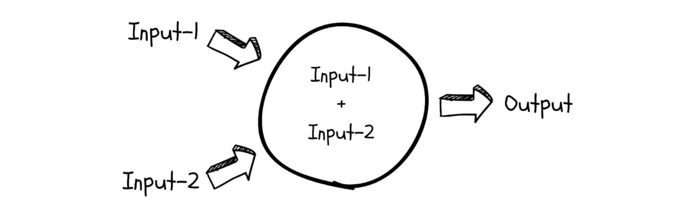
A neuron in software (also called a perceptron) is a deliberately crude imitation of the biological nerve cell in your brain. The biological neuron receives signals through its dendrites, mixes them, and either fires or doesn't fire down its axon. The software version does the same thing, just with arithmetic.
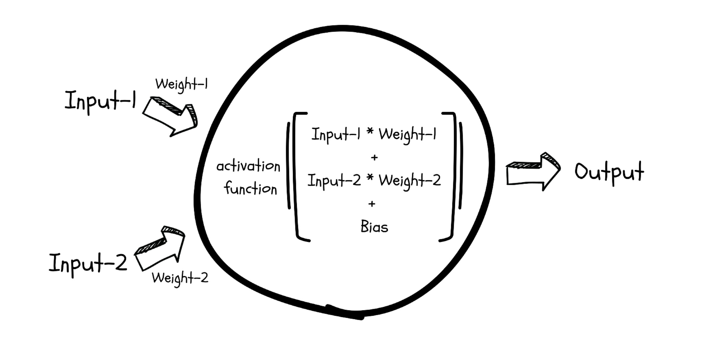
Mechanically, a neuron is just a small linear equation. It takes one or more numerical inputs, multiplies each input by a number called a weight, adds a constant called a bias, and produces an output:
$$ y = w_1 x_1 + w_2 x_2 + \dots + w_n x_n + b $$
You can read this as: "How much does each input matter (weights), and what's our baseline (bias)?"
The neuron's job: approximate a function
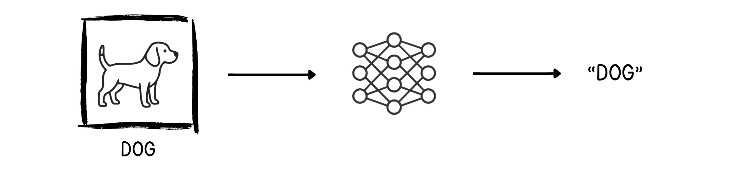
A neuron's purpose is to approximate the function that connects its inputs to its output. Think of a function as a rule like "given the pixels of this image, output 1 if it's a dog and 0 if it's a cat." Some rules are simple, some are mind-bogglingly complex.
Here's the catch: a plain linear equation can only draw straight lines. Most real-world rules — recognizing faces, translating language, predicting stock prices — are not straight lines. They bend, twist, and have thresholds. So the neuron needs a way to introduce non-linearity.
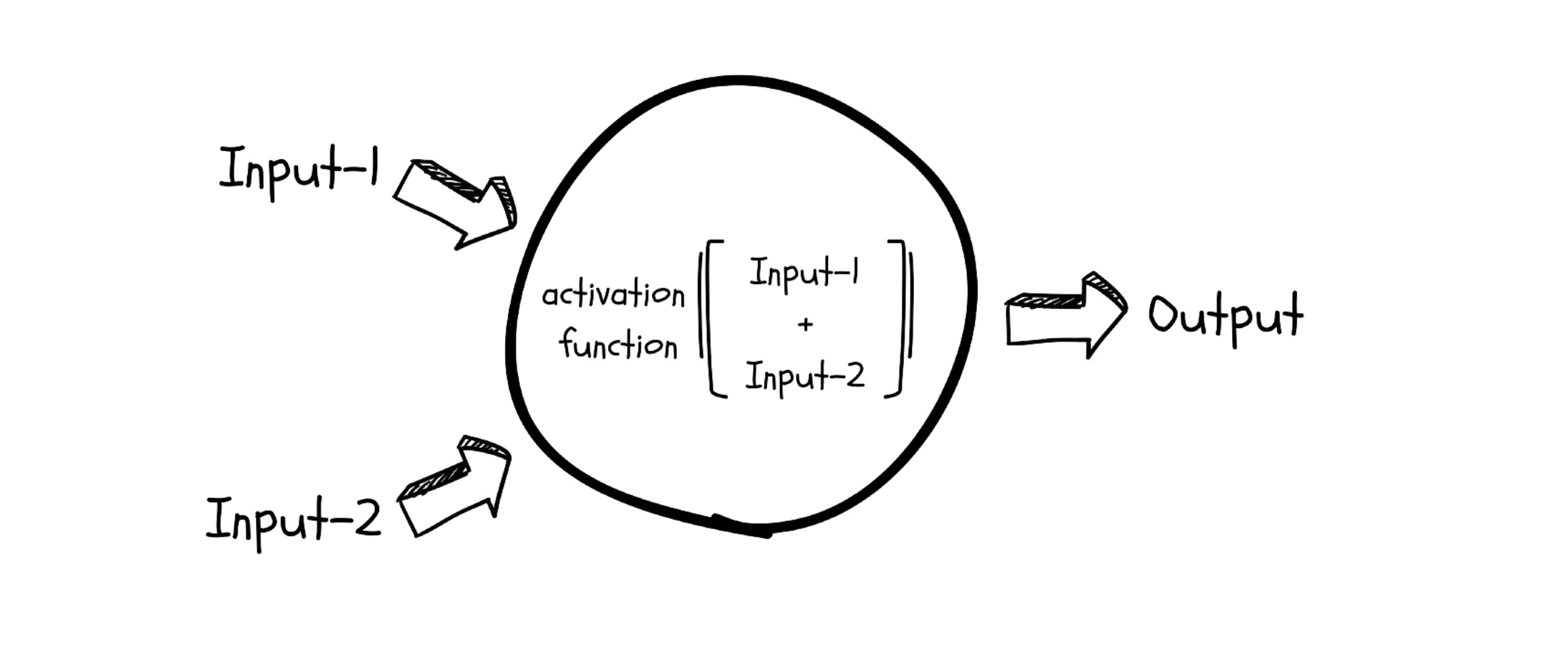
Activation functions: the bend in the line
After computing the linear sum, the neuron passes the result through an activation function — a small mathematical squisher that bends the otherwise-straight output into a curve. Without it, no matter how many neurons you stack, the whole network would still only be able to represent straight-line relationships.
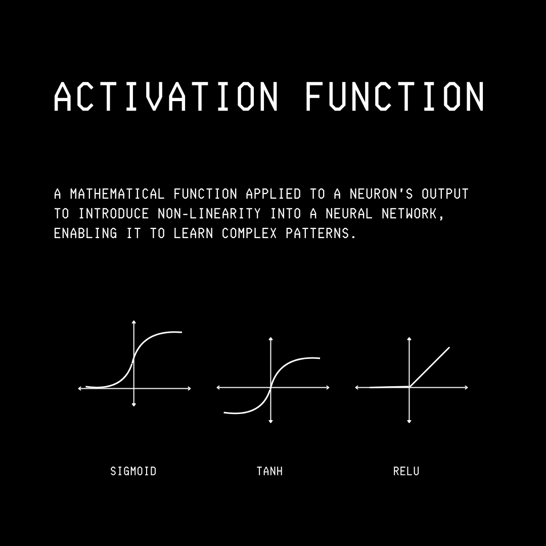
The three activation functions you'll see most often:
- Sigmoid — an S-shaped curve that squashes any input into a number between 0 and 1. Useful when you want to interpret the output as a probability.
- TanH — also S-shaped, but squashes between -1 and +1. Centered around zero, which often helps training.
- ReLU (Rectified Linear Unit) — the simplest of the three. If the input is positive, pass it through unchanged; if it's negative, output 0. Cheap to compute and surprisingly effective, which is why it dominates modern networks.
2. How does a single neuron learn?
The weights and biases inside a neuron are not fixed. They start out random — basically gibberish — and the whole point of "learning" is to nudge them toward values that make the neuron's output match reality.
But one neuron alone is a weak learner — it can only express simple relationships. The real power shows up when you connect many of them together.
3. Stacking neurons into a network
Connect multiple neurons in layers, where the output of every neuron in one layer feeds into every neuron in the next, and you get a neural network. Because every neuron is connected to every neuron in the adjacent layer, these are called dense layers (the alternative — sparse layers — is a story for another day). Because the architecture is many layers of perceptrons, it's also called a Multi-Layer Perceptron (MLP).
In the article's example, 5 neurons are arranged in 3 layers:
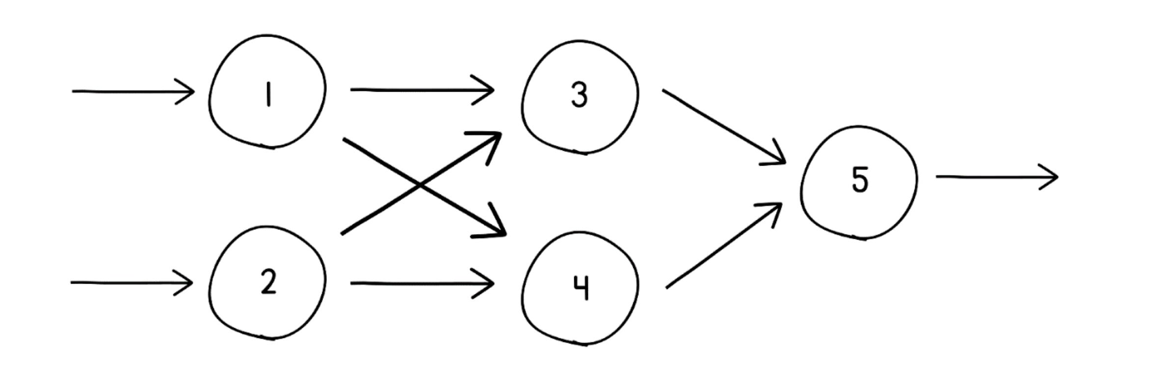
The layers have specific roles:
- Input layer — receives the raw input (e.g., neurons 1 and 2).
- Hidden layer — does most of the heavy lifting (neurons 3 and 4). It's called "hidden" because it sits between input and output and you usually don't inspect it directly.
- Output layer — produces the final answer (neuron 5).
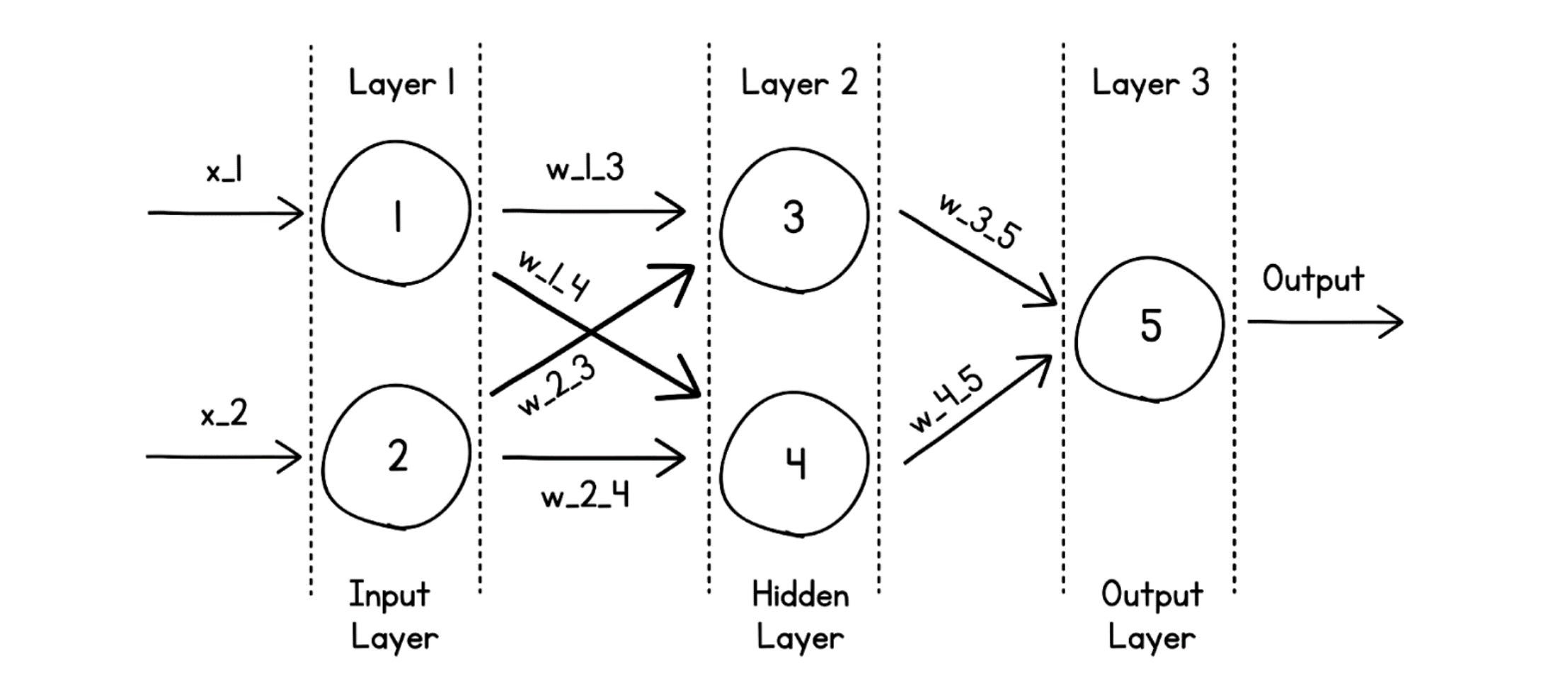
Zoom in on any single neuron and the same arithmetic from Section 1 plays out: each neuron has its own weights and bias, multiplies the values it receives, sums them, applies its activation function, and passes the result onward.
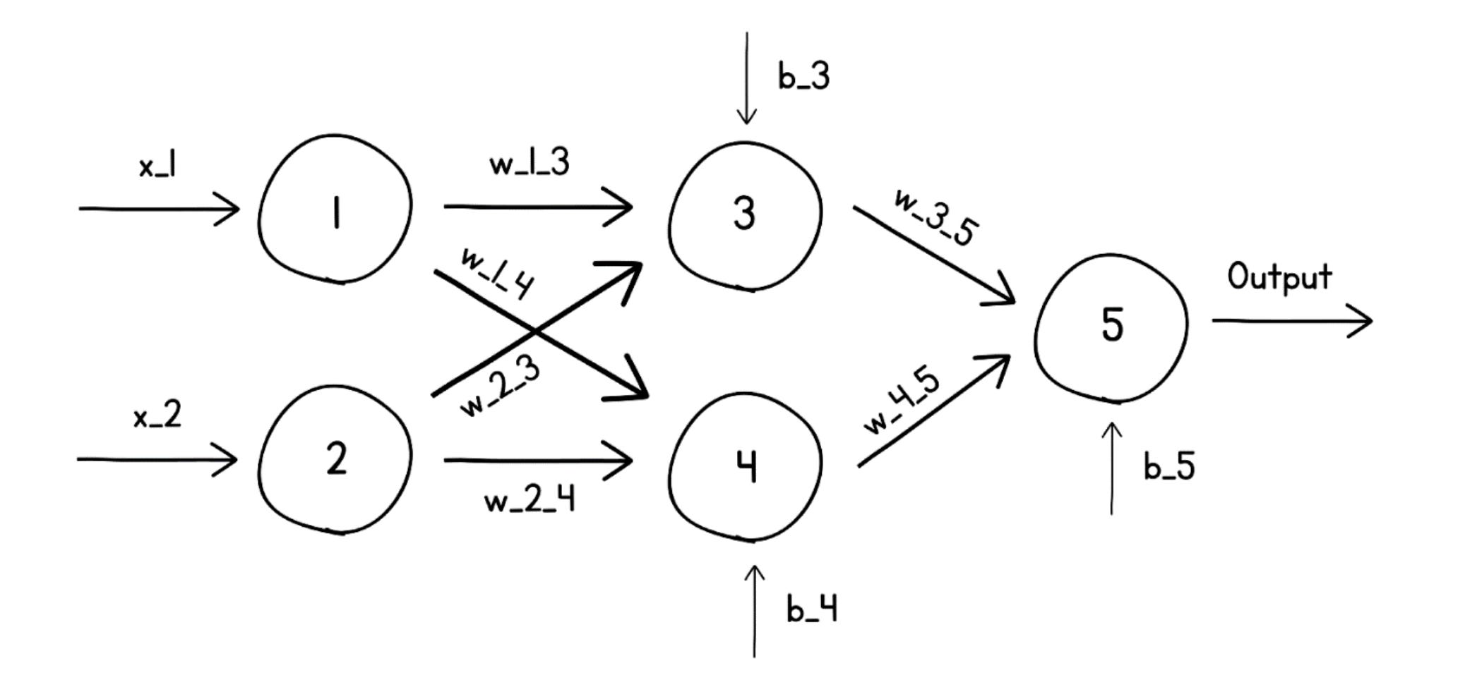
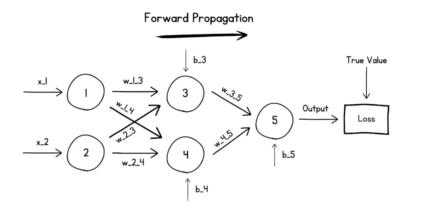
This calculation cascades layer by layer until the output layer produces the network's prediction. The whole left-to-right computation is called the Forward Pass (or Forward Propagation). And because data only flows in one direction — input to output, never looping back — this kind of network is called a Feed-Forward Network. (The alternative, Recurrent Neural Networks, do loop back; they're not covered here.)
4. How does the whole network learn?
Learning is an iterative loop where the network gradually adjusts every weight and bias in every neuron until its output matches the truth.
When training begins, all those weights and biases are random, so the first prediction is nonsense. The trick is: we already know the right answer for each training example (that's what makes it "supervised" learning), so we can measure how wrong the network is.
Step 1 — Measure the error with a Loss function
A loss function is a formula that compares the predicted output to the true value and returns a single number — the loss — that quantifies the mistake. Higher loss = more wrong.
Three loss functions you'll see constantly:
- Mean Absolute Error (MAE) — average of the absolute differences between predicted and true values. Used for regression (predicting numbers like prices).
- Mean Squared Error (MSE) — average of the squared differences. Also for regression. Squaring punishes big errors more than small ones.
- Binary / Categorical Cross-Entropy — used for classification, where the output is a probability between 0 and 1 (e.g., "85% chance this is a dog").
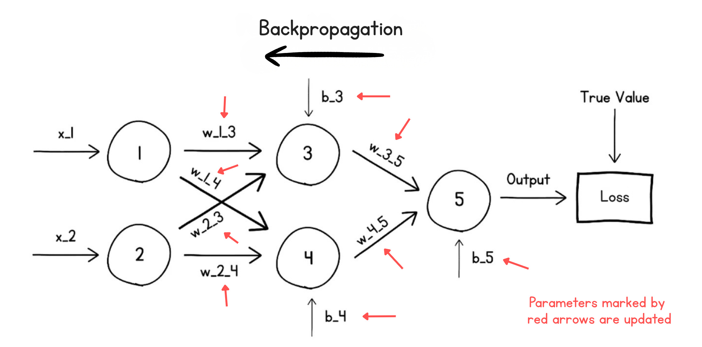
Step 2 — Push the blame backward (Backpropagation)
Now we know the network was, say, wrong by a loss of 4.7. Who's to blame? Some neurons contributed a lot to that error; others barely mattered.
Backpropagation (or the Backward Pass) is the algorithm that figures this out. It walks the loss backward through the network, layer by layer, and computes how much each individual weight and bias contributed to the total error. Each parameter is then nudged in proportion to its share of the blame, in the direction that will reduce loss next time.
Step 3 — The Optimizer decides how to nudge
The actual rule for updating parameters is called an optimization algorithm or optimizer. The article names three commonly used ones:
- Gradient Descent — the classic. Take a small step downhill on the loss landscape.
- Adam — an adaptive version that keeps a running memory of previous gradients, so it doesn't over-react to noisy single-step signals. Workhorse of modern deep learning.
- Muon — a newer optimizer.
Step 4 — Don't take giant steps (Learning rate)
The learning rate is a small multiplier (often 0.01, 0.001, etc.) that scales every parameter update. It's the brake pedal: too large and the network overshoots and oscillates wildly; too small and training crawls. Tuning the learning rate is one of the most important knobs in training.
Step 5 — Repeat, a lot
A forward pass + backward pass = one training step. You run thousands or millions of these. Each iteration, the loss decreases a little, until it's small enough that the network's predictions are very close to the true values. Training is done.
5. Worked example: cat vs. dog classifier
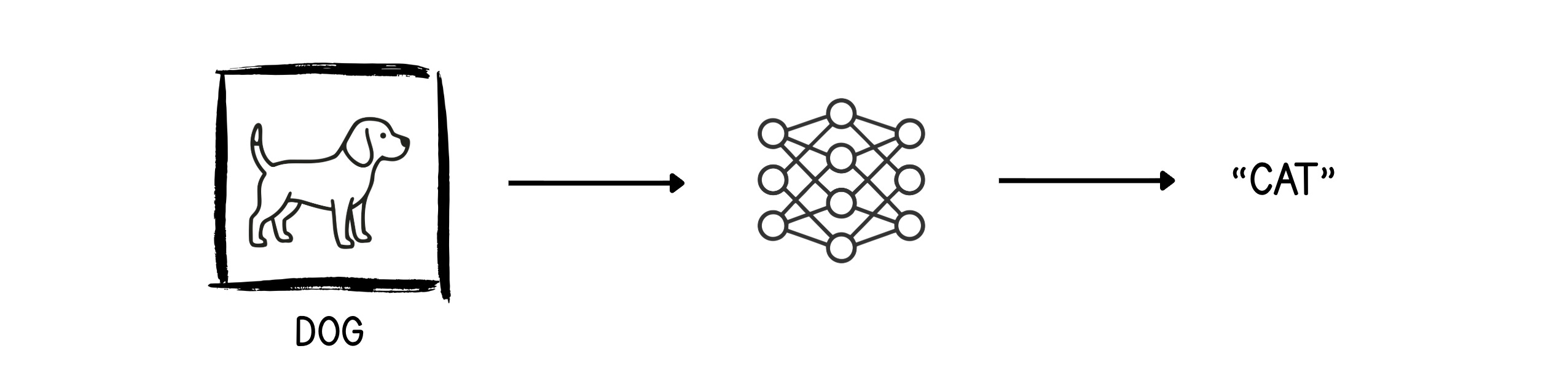
Concrete example to tie everything together. Goal: feed the network an image and have it output "Cat" or "Dog."
You start with a large dataset of labeled cat and dog images. For each image:
-
Forward pass — feed the pixels in. The untrained network, with random weights, makes a wild guess. Suppose it sees a dog image and confidently outputs "Cat." Wrong.
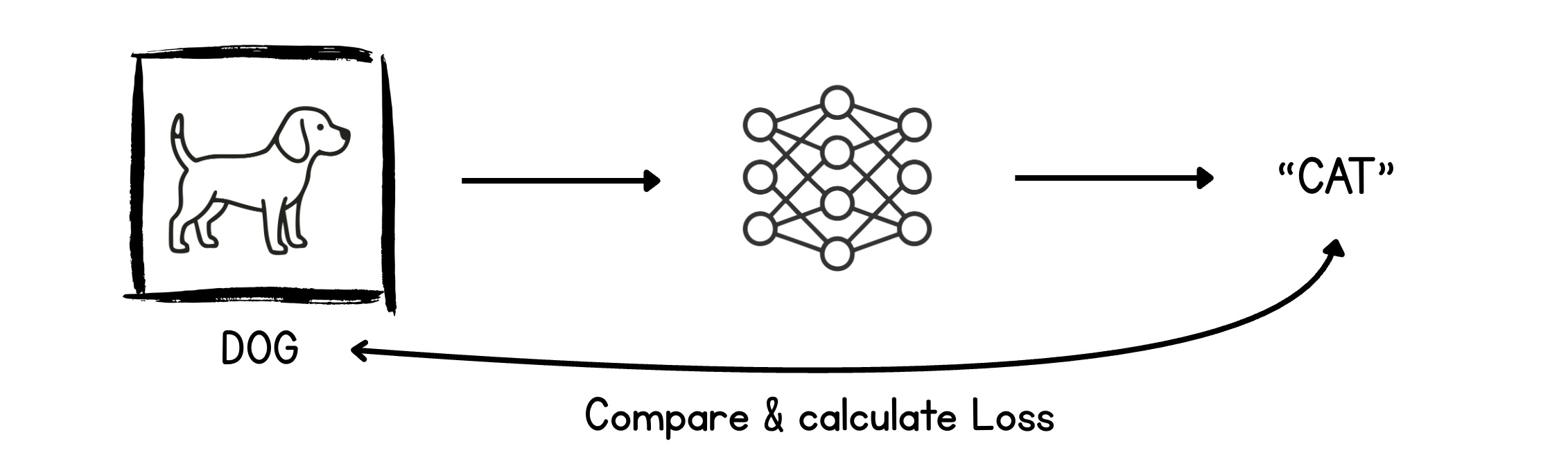
-
Compute loss — compare the prediction "Cat" to the true label "Dog" using a loss function, which spits out an error value.
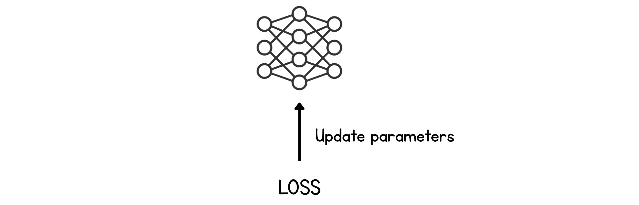
-
Backward pass — distribute that loss backward and update every weight and bias slightly, in the direction that would make the next prediction less wrong.
-
Repeat with the next image (and the next, and the next…). Eventually, the network sees a dog image and correctly outputs "Dog." Same goes for cat images.
When the network reliably predicts the correct labels across the dataset, training is complete.
TL;DR mental model
- A neuron = a tiny linear equation (weights × inputs + bias) followed by an activation function that adds a bend.
- Stack neurons into layers (input → hidden → output) and you get a neural network / MLP.
- A forward pass computes a prediction; a loss function measures how wrong it is.
- A backward pass spreads the blame; an optimizer (Gradient Descent, Adam, Muon) nudges every weight and bias by a tiny amount, scaled by the learning rate.
- Repeat for many iterations. Loss shrinks. The network has learned the function mapping inputs to outputs.
That's the entire foundation under modern AI — every Transformer, every diffusion model, every recommender system is just this loop, scaled up massively and arranged in clever shapes.
Author
Ashish Pratap Singh & Dr. Ashish Bamania
Continued reading
Keep your momentum
MKT1 Newsletter
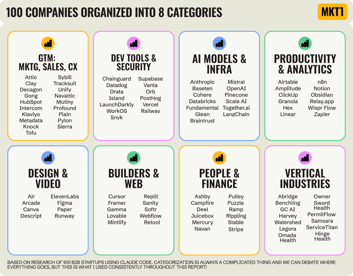
100 B2B Startups, 100+ Stats, and 14 Graphs on Web, Social, and Content
This is Part 2 of MKT1's three-part State of B2B Marketing Report. Where Part 1 looked at teams and leadership , Part 2 turns to what marketing teams are actually doing — what their websites look like, how they use social, and what "content fuel" they're producing. Emily Kramer u
Apr 28 · 10m
Lenny's Newsletter (Lenny's Podcast)
Why Half of Product Managers Are in Trouble — Nikhyl Singhal on the AI Reinvention Threshold
Nikhyl Singhal is a serial founder and a former senior product executive at Meta, Google, and Credit Karma . Today he runs The Skip ( skip.show (https://skip.show)), a community for senior product leaders, plus offshoots like Skip Community , Skip Coach , and Skip.help . Lenny de
Apr 27 · 7m

The AI Corner
The AI Agent That Thinks Like Jensen Huang, Elon Musk, and Dario Amodei
Dominguez opens with a claim that is easy to skim past but worth stopping on: the difference between elite founders and everyone else is not raw IQ or speed — it is that each of them has internalized a repeatable mental procedure they run on every important decision. The procedur
Apr 27 · 6m